Whiteboard Drawing Bot - Part 2: Algorithms

Daniel D. Johnson • 2014-08-04

In order to actually use my whiteboard drawing bot, I needed a way to generate the commands to be run by the Raspberry Pi. Essentially, this came down to figuring out how to translate a shape into a series of increases and decreases in the positions of the two stepper motors.

The mechanical design of the contraption can be abstracted as simply two lines: one bound to the origin point and one attached to the end of the first. The position of the pen is then the endpoint of the second arm:

The arms cannot move freely, however. The first arm can only be at discreet intervals, dividing the circle into the same number of steps as the stepper motor has. The second arm can actually only be in half that many positions: it has the same interval between steps, but can only sweep out half a circle. Furthermore, the second arm's angle is relative to the first's: if each step is 5 degrees and the first arm is on the third step, then the second arm's step zero follows the first arm's angle and continues at 15 degrees.

If you plot every point reachable by this apparatus, you get a pattern of dots similar to this:

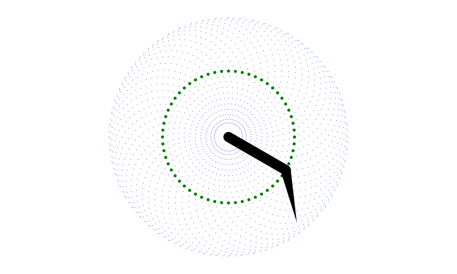
Notice that the second arm sweeps out half-circle arcs at each angular position of the first arm. This causes the resolution to increase close to the center and also near the outer edge.

This pattern is much more difficult to work with than a standard Cartesian grid: the two coordinates, position of arm 1 and position of arm 2, are not linear but circular. This poses some problems for rendering graphics.

Step position

We should probably start by figuring out the position of any given coordinate pair of integer steps $(s_1,s_2)$. To do this, we can add the x and y components of the two arm vectors, like so:

\[x=r_1*\cos(s_1\cfrac{2\pi}{steps}) + r_2*\cos((s_1+s_2)\cfrac{2\pi}{steps})\] \[x=r_1*\sin(s_1\cfrac{2\pi}{steps}) + r_2*\sin((s_1+s_2)\cfrac{2\pi}{steps})\]

Closest Point

An essential requirement before we can begin to draw anything is being able to find the closest reachable position from any point. Unfortunately, this calculation is not as simple as other coordinate system conversions, as the arms may be different lengths and do not depend on basic trigonometric equations. I ended up using the Law of Cosines.

Let us call the point we are attempting to approximate $P$. Then, one of three things is true:

If the distance between $P=(x,y)$ and the origin $(0,0)$ is greater than $r_1+r_2$ (the lengths of each arm), we know that the point is past the reach of the two arms. $\theta_2$ must equal $0$ and $\theta_1$ must equal $atan2(y,x)$. ($atan2$ is a function that returns the inverse tangent from $0$ to $2\pi$.)
Similarly, if the distance between $P=(x,y)$ and the origin $(0,0)$ is less than $r_1-r_2$, it is past the reach of the two arms. $\theta_2$ must equal $\cfrac{steps}{2}$ and $\theta_1$ must equal $atan2(y,x)$.
If the distance is between those two values, it is theoretically within reach of the arms. This requires more work to calculate.

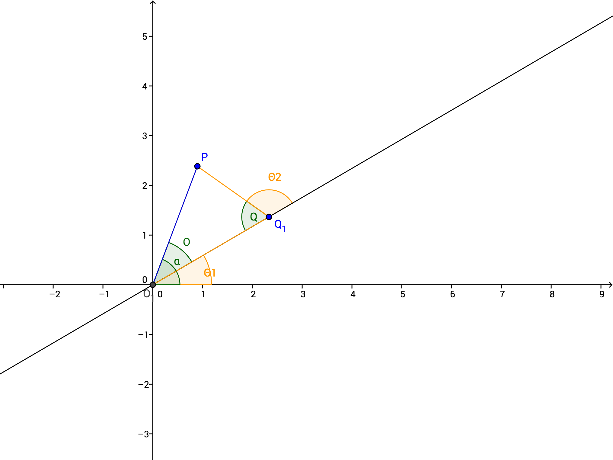
Note: As we are working in a computer graphics coordinate system to start, the y-axis is flipped and increases downward. This means that, among other things, an increasing angle moves clockwise, not counterclockwise, around the circle. Thus increasing steps move the arms clockwise as well. This means that the arms appear to bend the "wrong way" in this image, which uses the mathematical conventions.

For the third case, we know there exists a triangle that connects the origin $O$, the desired point $P$, and another point $Q$ such that $p=dist(O,Q)=r_1$ and $o=dist(Q,P)=r_2$. We can also calculate the distance $q=dist(P,Q)$ using the distance formula: $\sqrt((x_1-x_0)^2+(y_1-y_0)^2)$. Thus, we know all three arm lengths. By the Law of Cosines, we can calculate the angle measure of $Q$ and $O$:

\[\cos(Q)=\cfrac{p^2+o^2-q^2}{2po}\] \[\cos(O)=\cfrac{p^2+q^2-o^2}{2pq}\]

Then, we know that $\theta_1=atan2(y,x)-O$ and $\theta_2=\pi-Q$.

Finally, once we have finished calculating $\theta_1$ and $\theta_2$, we can calculate the step positions by rounding them to an integer step. If this is one of the first two cases, we can simply round to the closest integer step, like so: $s_1 = round(\theta_1*\cfrac{steps}{2\pi})$. If this is the third case, however, the rounding may not give the best results: we would not be finding the closest point according to Euclidean distance, but instead according to some strange double-angular distance function. We can, however, be confident that the desired point lies within the quadrilateral formed by rounding each value either up or down. (For example, if the ideal $s_1$ is 12.4 and the ideal $s_2$ is 60.25, the four points of the quadrilateral are $(12,60)$, $(12,61)$, $(13,60)$, and $(13,61)$.) Thus, we calculate those four potential approximate points and pick the one with the smallest distance. (Note: As we only care about relative distance, we do not have to take the square root. We can instead simply compare distance-squared: $(x_1-x_0)^2+(y_1-y_0)^2$)

Lines and Curves

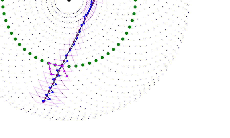
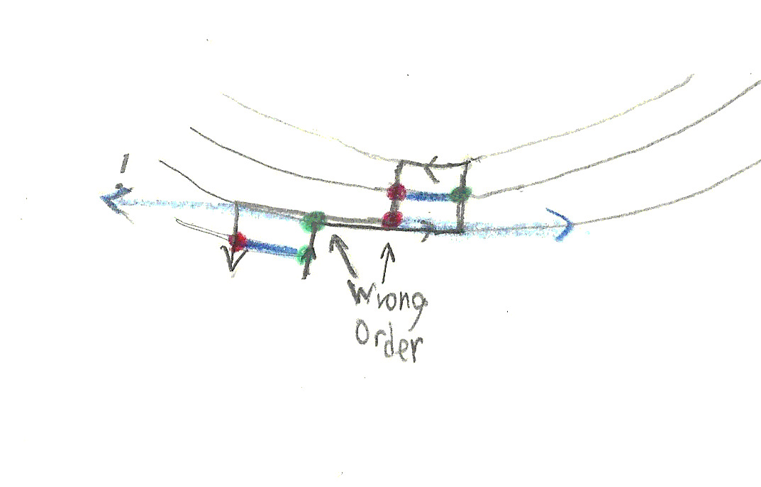
Now that we can find the closest position to a point, how do we draw lines and curves? A naive approach would be to sample the curve at various points and choose the closest position at each. This is problematic for a few reasons. First of all, the path chosen would likely not be the best path. As the reachable points are not distributed evenly, jumping from closest point to closest point produces a jagged, uneven curve that does not behave in the way we would like. Ideally, we want the approximate path to move in the same direction as the line or curve. Furthermore, that path must move with only 1-step intervals, a condition not necessarily guaranteed by the closest-point algorithm, especially near the edges of the drawable region. (Also, sampling points is kind of messy, and with Bezier curves the time steps do not directly correspond to progress along curve, meaning we would need to do complex calculations just to figure out where best to sample.)

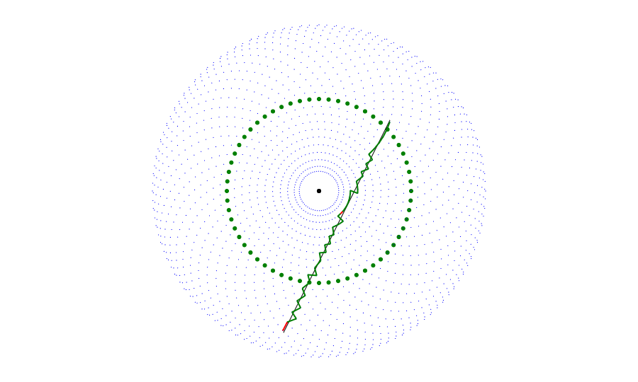
Notice how the path is very jagged and does not follow the line's direction. Furthermore, there are two instances (colored red) where the path skips over steps, making it impossible to draw.

Instead of sampling points, I decided to design a different algorithm. My algorithm works under the assumptions that:

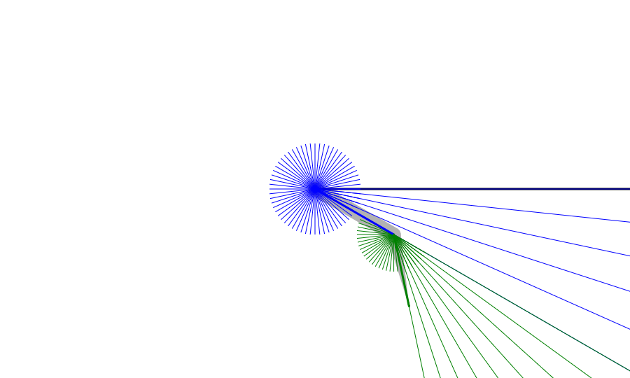
From any given point, there are eight possible positions that can be reached: increasing or decreasing the first arm's step position, increasing or decreasing the second arm's step position, and moving both arms simultaneously.
The approximation should preserve the overall shape of the curve. Thus, capturing small variations is less important than capturing the curve's overall direction.
The curve is continuous and can be described by a mathematical equation.

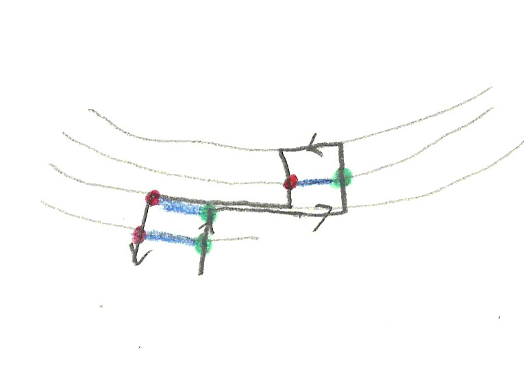
The basic procedure is as follows: 1. Find the steps closest to the starting point of the curve. Set curstep to this value. Also set progress to 0. 2. Find all eight points that can be reached from this step. Arrange them into an octagon. 3. Intersect each of the sides of this octagon with the curve. Collect the points that intersect farther than progress along the curve. If there are multiple intersections that fit this critera, take the one closest to the current progress. 4. If an intersection was found, take the side of the octagon that was hit and find which of the two points on that side is closest to the intersection. This is the new curstep position, and progress is the found intersection's progress along the curve. Repeat from 2. 5. If no intersection was found, the curve ends within this polygon. Find the closest position to the curve endpoint.

After this procedure, iterating along the curstep values will form the best approximation of the curve.

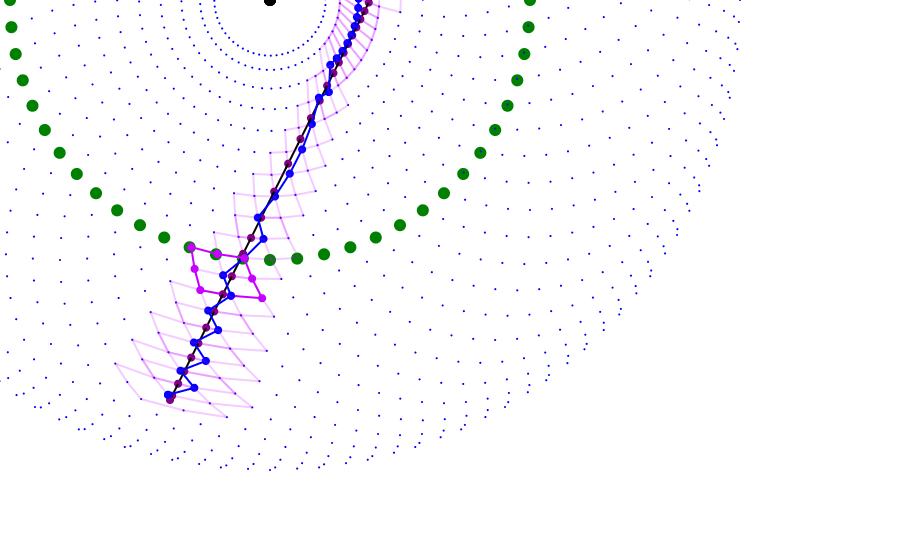
This algorithm works because it essentially chooses at each step the arm movement that approximates the curve's motion. By only choosing the next point once the curve passes through a gap between two other positions, the approximation is able to show the overall direction of the curve instead of the particulars.

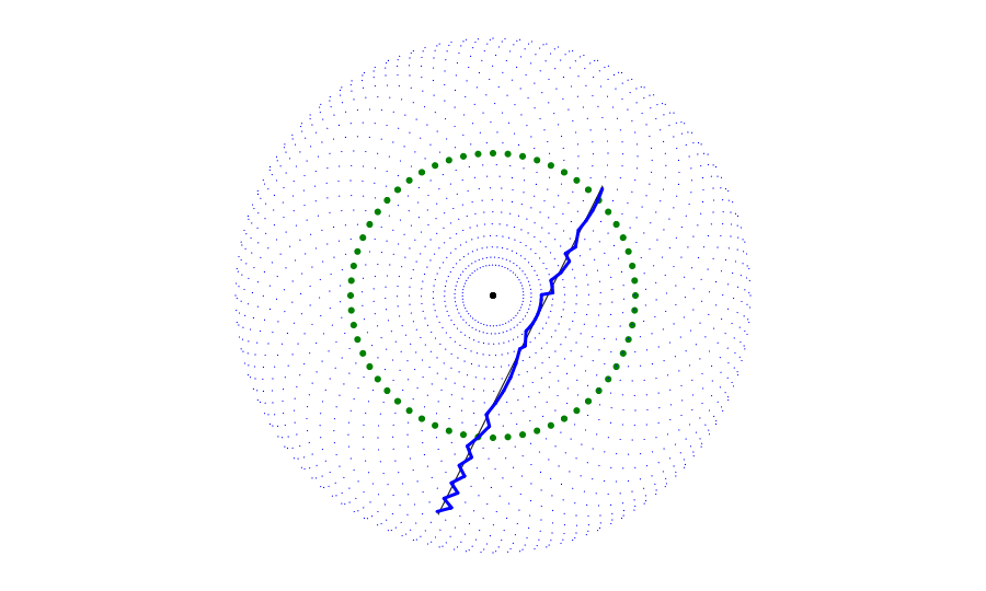
Notice that the final result does not have as many jagged edges (although it does have some) and that it does not jump to any point that is unreachable.

Note: In order to handle lines and curves that exit the drawable boundary, I implemented "special" adjacent points for when the current second-arm step is at either 0 or steps/2. At 0, the "adjacent" point is 10x as far as the contraption's radius, and at steps/2 it is at the origin. This enables the algorithm to handle extending paths without much difficulty: it snaps to the farthest possible points and never goes further.

Filling it in

The above algorithm allows me to generate a path that approximates any shape. (Well, theoretically. I have only implemented intersection code for straight lines and cubic Bezier curves. But that is enough for my purposes.) Stroking those shapes is easy; just follow the path. Filling them in, however, is harder.

In graphics, there are a few different conventions for determining whether a point is inside or outside a polygon. The even-odd rule states that if you pass an odd number of edges as you go from the point out of the shape, the point is inside. If the number is even, it is not. The nonzero winding rule states that if there is a nonzero difference between the number of times you hit an edge that goes counterclockwise and the number of times you hit one that goes clockwise, the point is inside. This situation is different, however, from a normal scenario. We are not judging points individually. Instead, we want to draw lines across the shape. Because of the cyclical nature of the drawing space and the other intricacies, I made some more simplifications and assumptions.

I assumed that all shapes satisfy the following properties:

They are made of a series of paths. Each path ends at its starting point and does not intersect itself.
None of the paths intersect each other.
Any path that is within another path is oriented in the opposite direction (for example, a path inside a clockwise path goes counterclockwise)
Any path that is not within any other path is oriented counterclockwise.

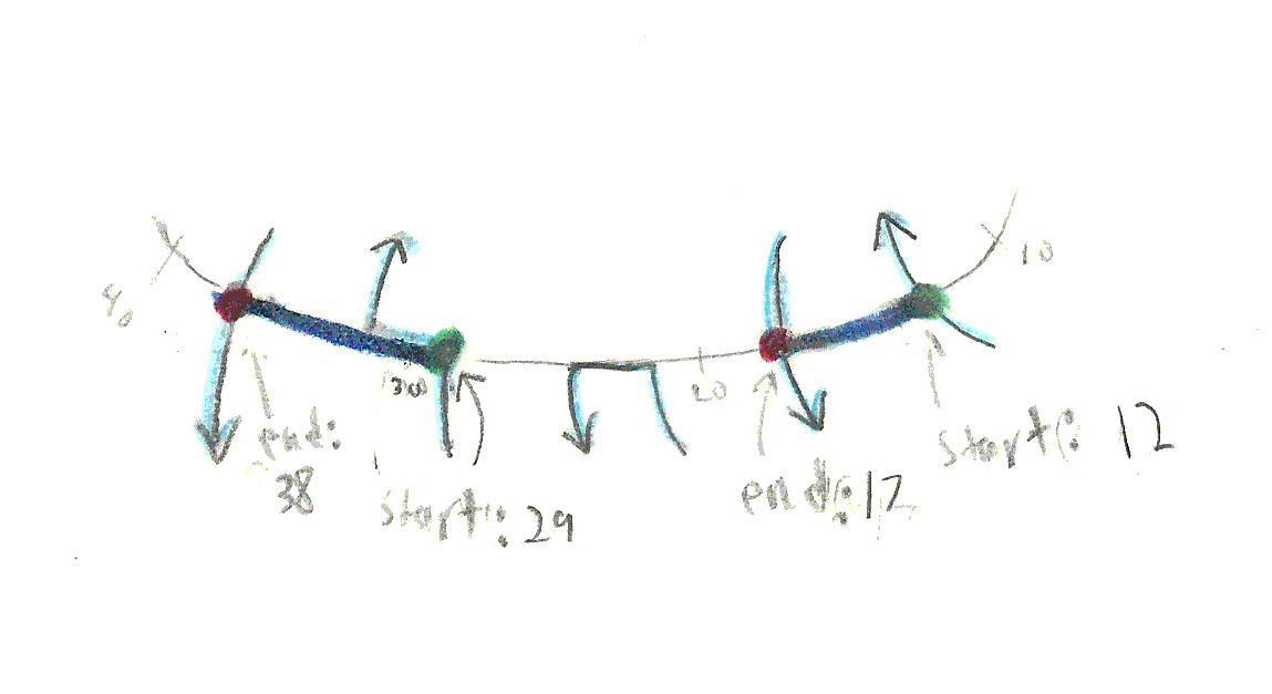
With these assumptions, I can calculate the fill regions by creating a table of all the second arm's positions (which correspond roughly to radii, but in the opposite direction) and keep track of the first arm positions (which correspond roughly to angular position, clockwise) where a path crosses through each second arm position. If the second's position is increasing, that first arm position is the start of a fill region. If the second's position is decreasing, it is the end of a fill region.

One thing I had to watch out for was what to do when the path stays at the same secondary position for multiple points in a row. My first implementation simply took the start and end points as being the primary position when the path first reached that secondary position, but this caused problems. Sometimes, starts and ends would get out of order!

I solved this by always taking the first intersection if the second arm is increasing and the last intersection if it is decreasing. That ensures that the endpoint is always after the startpoint on a non-self-intersecting curve.

I also combined multiple starts and ends happening at the same coordinate to eliminate errors at those points. If there are more starts than ends it becomes a start, if there are more ends than starts it becomes an end, and if they are the same they are all removed.

To change the fill density, I check if the secondary position mod interval is zero, where interval is the interval at which lines should be drawn to fill the shape.

To actually translate fills into a command, I iterate through the secondary angles, sweeping the pen back and forth across the affected area and lowering/raising the pen at each start/end point, respectively.

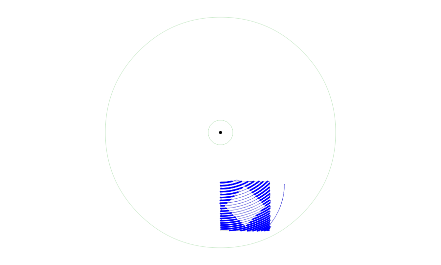(The thin blue lines mark the path of the pen head as it moves from position to position without writing)

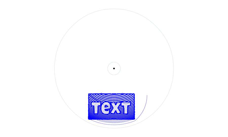
Text

From the beginning, I wanted to add text support to the shape generator. Luckily, I found opentype.js, a Javascript parser for OpenType and TrueType fonts. One caveat was that many fonts use quadratic curves, not cubic ones. In order to avoid having to check if they were cubic or quadratic throughout my code, I translate the quadratic curves into cubic curves and then treat them like cubic curves everywhere. If a quadratic curve is defined by points $Q_0$, $Q_0$, and $Q_0$, then the corresponding points for the cubic are:

\[C_0 = Q_0\] \[C_1 = Q_0 + \cfrac{2}{3}(Q_1-Q_0)\] \[C_2 = Q_2 + \cfrac{2}{3}(Q_1-Q_2)\] \[C_3 = Q_2\]

One problem, however, was that I was using a cubic root equation to find the intersections between the curves and the lines. A quadratic curve has a zero cubic term, even if it has been turned into a cubic curve. I thus implemented a fallback quadratic equation solver if the cubic term is zero. In fact, I had to implement a linear solver because some fonts had straight lines made out of quadratic curves! Ultimately, however, I was able to use the font paths just like any other shape path, and so the same approximation and filling algorithms I made for simple shapes work seamlessly with textual input.

Thanks for reading! If you missed the mechanical construction of the bot, you can read about it in the first part of this series. You can also read the next part, in which I discuss the simulator and shape editor interface!