Summer Research on the HMC Intelligent Music Software Team

This summer, I had the chance to do research at Mudd as part of the Intelligent Music Software team. Every year, under the advisement of Prof. Robert Keller, members of the Intelligent Music Software team work on computational jazz improvisation, usually in connection with the Impro-Visor software tool. Currently, Impro-Visor uses a grammar-based generation approach for most of its generation ability. The goal this summer was to try to integrate neural networks into the generation process.

Product-of-Experts Generative Model

The first major project was building a generative model, similar to the work I did with polyphonic music in an earlier blog post. However, there are some differences between modeling polyphonic music and modeling jazz solos for Impro-Visor.

• Firstly, the polyphonic music task is polyphonic, i.e. there may be multiple notes playing at the same time. This was what enabled me to use the convolution-like parallel structure in my first network model. However, the jazz solos that Impro-Visor uses are monophonic.
• Additionally, when improvising a jazz melody, one has to follow an underlying chord progression. This was not present in the polyphonic task.

Since only one note is playing at a time, the network architecture can be much simpler. In particular, instead of having a different LSTM stack for every note, it is possible to use only a single LSTM stack. However, my work with polyphonic music showed that having a transposition-invariant architecture provides many benefits. In order to be transposition-invariant, we need to interpret the output of the network as being relative to something. But to what?

One candidate is the previous note. In effect, the network would be picking interval jumps from one note to the next. Such an architecture would be transposition invariant, since the sizes of intervals don't depend on absolute position. This would also help the network learn to make smooth contours.

However, another promising candidate is the current chord. Each part of the melody exists on top of some chord (generally played by the piano or bass). Modeling notes relative to a chord would again be transposition invariant, since the chords would also shift during a transposition. Furthermore, this would encourage the network to learn what kinds of notes are consonant with different chords, and which notes to avoid.

Since each of these have unique advantages, it would be great if there were a way to combine them. It turns out that such a way exists, and it is based on an idea by Geoffrey Hinton called product-of-experts.

Product-of-experts is a way to combine two simpler probability distributions into one distribution. The idea is to multiply together the density functions of each probability distribution, and then normalize the result so that it sums to 1. For example, if $P(x|E_1)$ is the chance of picking choice $x$ predicted by the distribution of expert 1, and $P(x|E_2)$ is the chance of picking choice $x$ predicted by that of expert 2, where $x$ is part of some larger set of choices $A$, we can compute the combined probability as

$$ P(x| E_1, E_2) = \frac{P(x|E_1)P(x|E_2)}{\sum_{y \in A} P(y|E_1)P(y|E_2)}. $$

One interesting thing to notice is that we can interpret this combination as a probabilistic "and" using the definition of conditional probability:

This is the basis for what we called the Product-of-Experts Generative Model of jazz improvisation. Basically, we trained two different LSTM networks, one to predict intervals, and another to predict notes relative to the chord. To train the model, we used product-of-experts to combine the probability distributions of the two networks, and then computed the likelihood of the correct note choice based on that product distribution.

The results from this are very promising, although they aren't quite as appealing as the melodies generated by Impro-Visor using grammars. They also produce some pretty cool graphs!

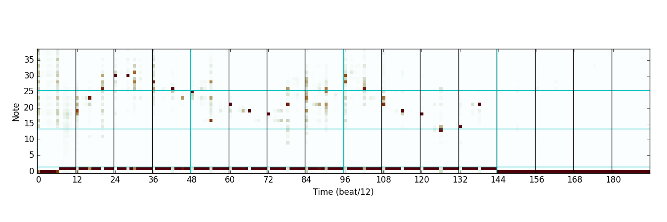
First, we have the distribution predicted by the interval expert network:

Notice that this network output seems to capture the idea of contour; its output is mostly smooth and controls the direction of motion. (Darker means more likely to choose that note.)

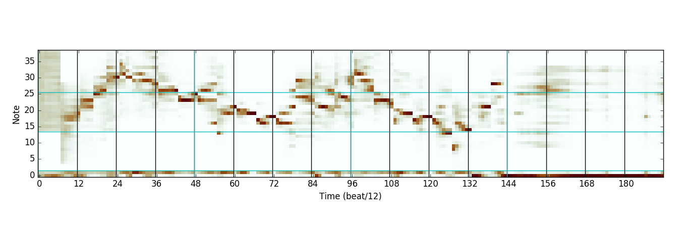
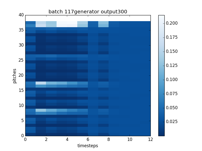
Next, we have the distribution predicted by the chord expert network:

There are a few things interesting about this output. First, it appears that the chord network also learned to model rhythm. (The bottom two lines represent chance to rest or sustain in the next timestep, and the rest represent chance to articulate a new note.) The fact that the chord network learned this appears to be arbitrary; in a different training run it was the interval expert that learned rhythm. The second thing that is interesting is that the chord network does seem to successfully identify some notes as being good choices to play over the chord and others as not.

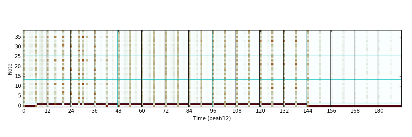
When we take the product of the distributions, we obtain this:

Notice how many fewer high-probability choices there are after the product operation. In essence, each expert can reject notes that it does not like, and only the notes that both experts think are plausible are kept.

Sampling from this distribution yields

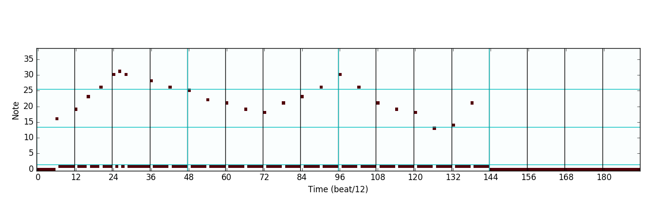
which can be viewed as notes on a staff:

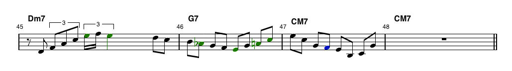
(Note: Technically, sampling occurs on a timestep-by-timestep basis. So the output for timestep 1 is sampled, and fed back into the networks before computing timestep 2.)

Compressing Sequence Autoencoder

The second model I worked on was called the Compressing Sequence Autoencoder. The motivation behind it was a specific type of improvisation called trading. Trading happens when there are two players that alternate playing short solos, usually of about 4 measures long. One type of trading is a sort of call-and-response, where one player plays a solo, and the next plays a variation of that solo that is slightly different but has a similar structure. We wanted to see if we could use a neural network to generate interesting variations on an input solo, and use that as a trading partner.

One naive way to generate variations of a solo would be to just adjust the notes a little bit. Maybe we'd shift some notes up or down, or move them around in time. However, the problem with this is that just moving the notes probably won't make a good solo. We want to somehow shift the solo within the space of good solos, so that we end up with a similar solo that is still an acceptable melody.

Based on some other research (such as this and this), one way of doing this is to train an autoencoder. An autoencoder is a type of neural network with two components: an encoder, which learns to convert the input into some encoded feature vector, and a decoder, which learns to reconstruct the input as well as possible from the feature vector.

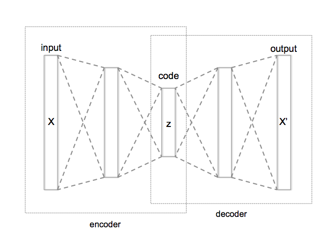
Assuming the autoencoder trains well, we can then perform our manipulations in the latent space of the encoded feature vectors. This allows us to do all sorts of things. We can add noise to an encoded input, essentially taking a random small step in feature space, and then decode the result to obtain a slightly different output. We can even interpolate from one input's code to another, obtaining a continuous progression of outputs from one to the other.

Importantly, however, jazz melodies are sequential in nature, and they have a very important temporal component. So we have to be careful how we apply autoencoders. In other research with sequential autoencoders, there are two main paradigms:

• Global autoencoders: Read in the entire sequence, create a single coded vector, and decode back to the entire sequence
• Timestep-level autoencoders: Encode a single timestep as a coded vector, and decode that timestep, then move to the next timestep conditioned on the result of the first.

Neither of these work well for jazz melodies. The problem with global autoencoders is that we want to be able to encode a melody of arbitrary length, but it isn't reasonable to expect the network to cram information about a long solo into a single fixed size vector. And the problem with timestep-level autoencoders is that they aren't usually designed to give a representation of a sequence as a whole.

Our solution was to combine the two approaches. Our autoencoder produces a sequence of encoded vectors, but this sequence must be shorter than the input sequence. In particular, we allow the autoencoder to output a single encoded feature vector for every half-measure worth of input. This allows us to handle arbitrarily long solos while also obtaining a sequence of vectors that together represent each part of the input melody.

The results after training this model are extremely exciting. We performed principal component analysis of the feature vectors across our entire input corpus and produced the following graph of the first 3 components:

Notice the three clusters. There's the main cluster around zero, which we would expect, since our data is relatively similar and thus should be close together in feature space. But importantly, there are also two other peripheral clusters. After investigation, we found that one cluster corresponds to measures that are just rests, and the other corresponds to measures that have long notes. Even more interesting is that, as shown by the colors of the points, the notes get progressively longer as we move from the rest cluster to the long note cluster. This means that the encoded feature space represents meaningful structural properties of our input data!

We can use this feature space to interpolate between different melodies. Here's the results of interpolating between two songs in our input corpus:

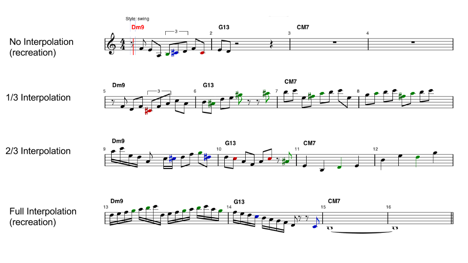
Notice that the solos in between are still viable jazz solos, but the structures of them shift relatively smoothly between the first solo and the last one.

There are a couple variations of this that we tried. At first, we thought we could get good results by allowing the encoder network itself to determine where to put the features, instead of forcing them to be output every half measure. However, what ended up happening is that the encoder figured out it could just output one feature at the start of each note. This of course allowed it to reconstruct the input very accurately, but wasn't really what we were going for. Another thing we are still working on is trying to use a larger dataset and variational inference to make a smoother and more complex feature space, but results from that are still being collected.

Generative Adversarial Model

One more thing that I'll touch on is the Generative Adversarial Model. I didn't work on the implementation of this directly, but I helped out with some of the design of the model. The idea was to try to extend the idea of generative adversarial networks to sequential music.

The basic idea behind generative adversarial models is to use two separate networks: a discriminator, which tries to tell the difference between the training data and generated data, and a generator, which generates new data and attempts to fool the discriminator into thinking the generated data is real. Generative adversarial networks seem to work best with continuous-valued input, but we thought it would be interesting to try to apply them to discrete sequences.

One of the issues we ran into was that in order to train the generator, we need to be able to backpropagate the discriminator output back through the discriminator. Equivalently, we need to be able to take the derivative of the discriminator's output with respect to the weights of the generator. This is problematic, since in order to generate a melody we need to sample from the generator's distribution, and sampling is discontinuous and not differentiable.

Our solution was to have the discriminator output a different score for each timestep, and then backpropagate the expected value of the discriminator's output using the generator's distribution from that timestep. This makes it fully differentiable, since the expected value is essentially a weighted sum. Then we can sample one particular output before moving on to the next timestep.

Unfortunately, it was very difficult to get the model to train effectively. The main problem we ran into was that the discriminator would decide very early on whether the input was real or generated. At the beginning of training, it would be clear which was which after only a few timesteps: the real data would generally play a note and then sustain it, whereas the untrained generator would play a bunch of random notes in quick succession. After seeing that, the discriminator learned to stop paying attention to later timesteps, and simply make its decision based on the first few. This meant that there was no real gradient for training the generator on the rest of the piece, only on the first few timesteps. As a result, the generator would slowly learn how to model the first few timesteps, but would not be able to learn the rest of the piece.

With continued work, it is likely that we could get the generative adversarial model working here. However, for discrete sequence data such as this, generative adversarial models have little advantage over regular generative models that predict a probability distribution. The real strength of generative adversarial models is with complex, high-dimensional continuous data, such as images, where evaluating a probability distribution is intractable. (For instance, here's a GAN learning to make bedrooms, faces, and album covers!)

Now what?

Right now, the work with the product-of-experts generative model has been integrated into the Impro-Visor project! If you are curious about the Theano code used to build the model, that is available on GitHub under the lstmprovisor-python repository. You might also be interested in the bleeding-edge version of the open-source Impro-Visor project, which is also on GitHub. (The version of the model in Impro-Visor is just generative; you need to use Python to train a new model. This is because we could not find any flexible machine-learning libraries in Java that were as easy to use as Theano is in Python.)

The code for the autoencoder is also in the first GitHub repository above, but the autoencoder-based active trading is still being implemented. Fairly soon, that should make its way into Impro-Visor as well, in time for the next release, and then anyone should be able to install Impro-Visor and play with the results! If you want, you can try using the models right now from Python, and you can also build Impro-Visor from source to try out the generative model integration. The input format for training is the Impro-Visor leadsheet format, with extension .ls, but Impro-Visor allows conversion to leadsheet files from MIDI or MusicXML, if you want to train with your own data.

Eventually, we hope to finish running the autoencoder experiments and then write a paper describing our work. We are currently planning to submit our work to the International Conference on Computational Creativity (ICCC) this year.